Womb

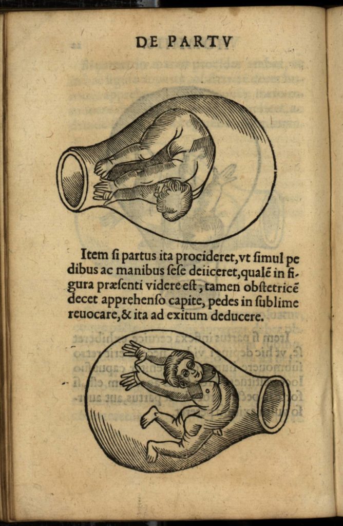
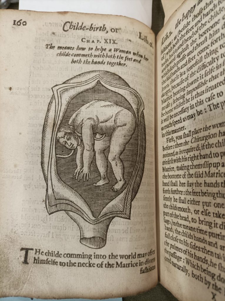
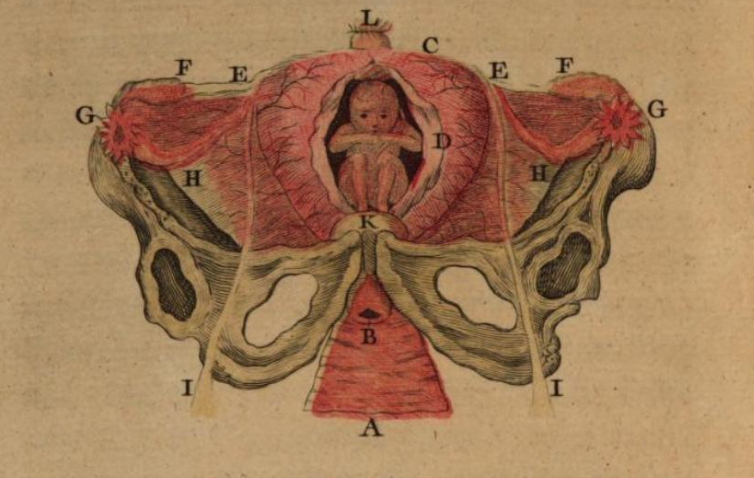
The Uterus is three inches long, from the Os internum to the upper part of the Fundus and one inch in thickness from the fore to the back-part […]. The shape of the Uterus, in some measures, resembles […] a kind of pear which hath a long neck”
(smellie, 1752/1974, p. 96)

The womb is perhaps the most important physical element of the female body we can examine and compare in our sources. For the authors under study, the womb was the locus of every ailment the female body could encounter and suffer.

Language to Describe the Womb 1532-1785

English sources

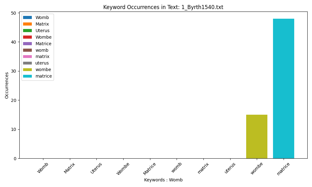
Byrth of Mankynde uses older spellings of both ‘womb’ and ‘matrix’, with ‘matrice’ being the preferred term for Roselin.

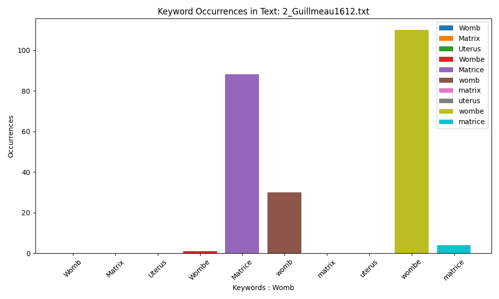
Guillemeau employs two spellings, introducing ‘womb’ without an ‘e’ to the corpus. He prefers ‘womb’ over ‘matrix’.

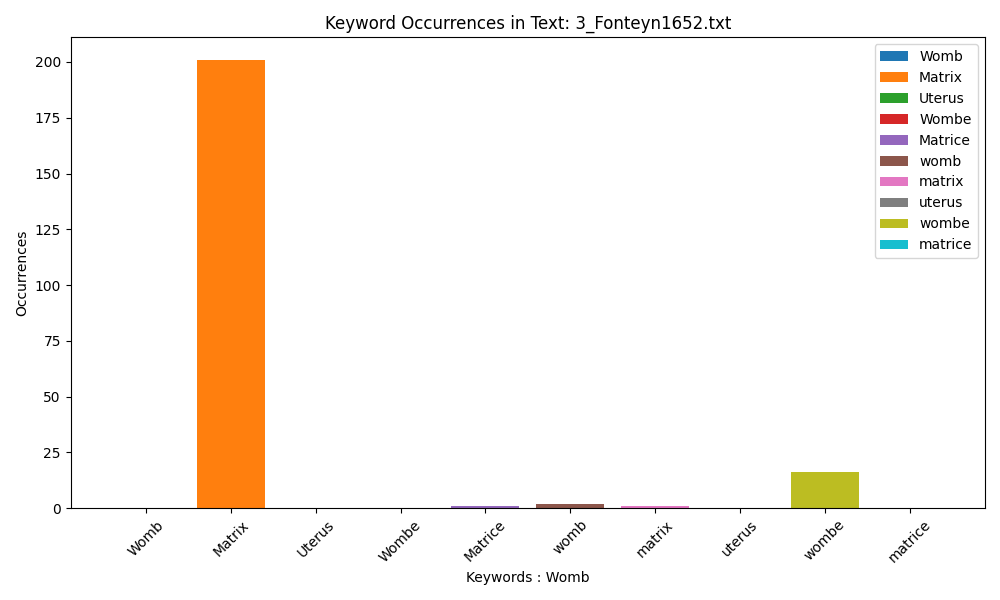
Fonteyn prefers ‘Matrix’ and ‘wombe’, a trend which highlights the difficulties in standardising medical langauge in the Early Modern era.

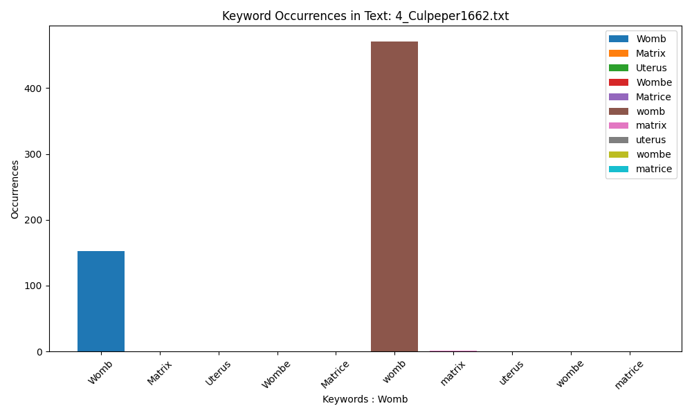
Culpeper’s use is more standardised and he uses exclusively ‘womb’, using it with both an upper and lower case spelling.

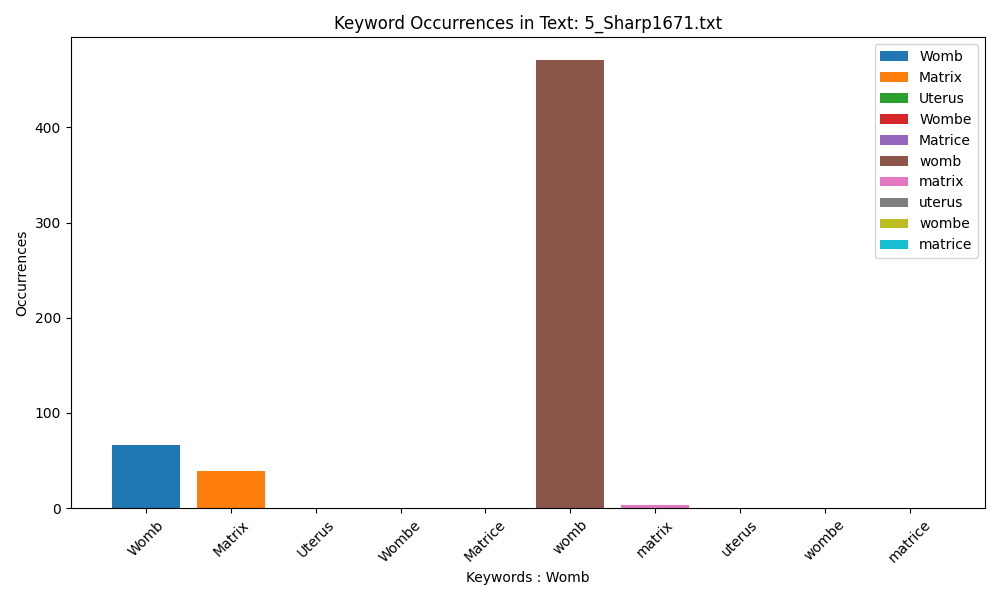
‘Matrix’ and ‘matrix’ are used sparingly by Sharp, who also uses a standardised form of ‘womb’. Both the length of her text and the importance she places on the womb as a point of discussion are noted here.

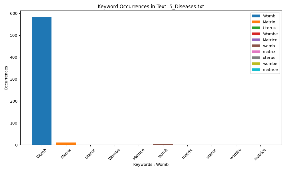
Diseases of Woman with Child (1672) employs ‘Womb’ 590 times, rarely in lowercase form. ‘Matrix’ is used seldomly.

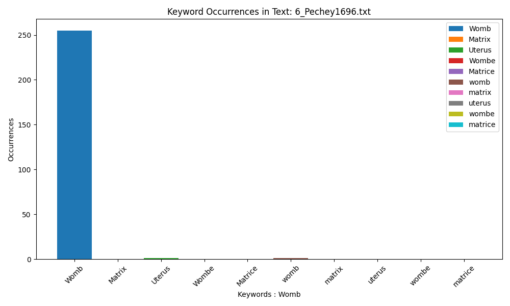
Pechey introduces ‘uterus’ to the corpus but seldom uses it.

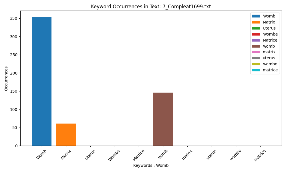
The use of ‘Matrix’ resurges at the end of the 17th century, but as The Compleat Midwife’s Practice is a compilation text harvested from earlier sources, this trend is unsurprising.

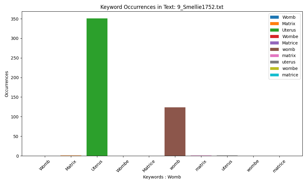
Smellie prefers ‘Uterus’, using it over 350 times, while ‘womb’ is also used relatively often.

French sources

The French sources display less of a variation; matrice is used almost exclusively.

Joubert uses ‘matrice’ exclusively.

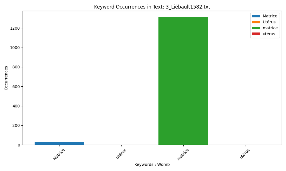
Liébault translates from Marinello using both ‘Matrice’ and ‘matrice’.

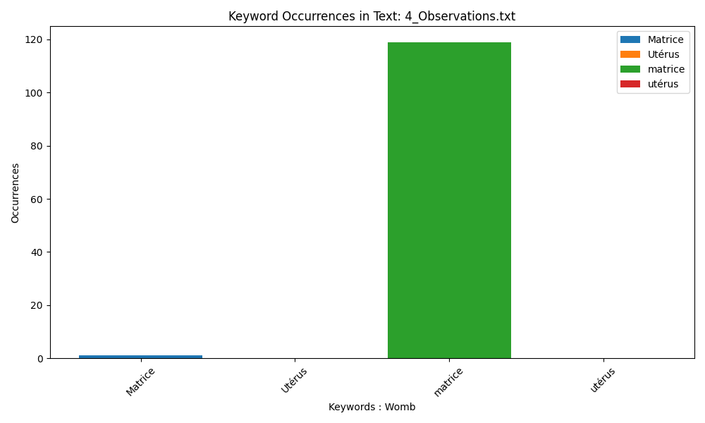
Lowercase ‘matrice’ is almost alway used by Bourgeois.

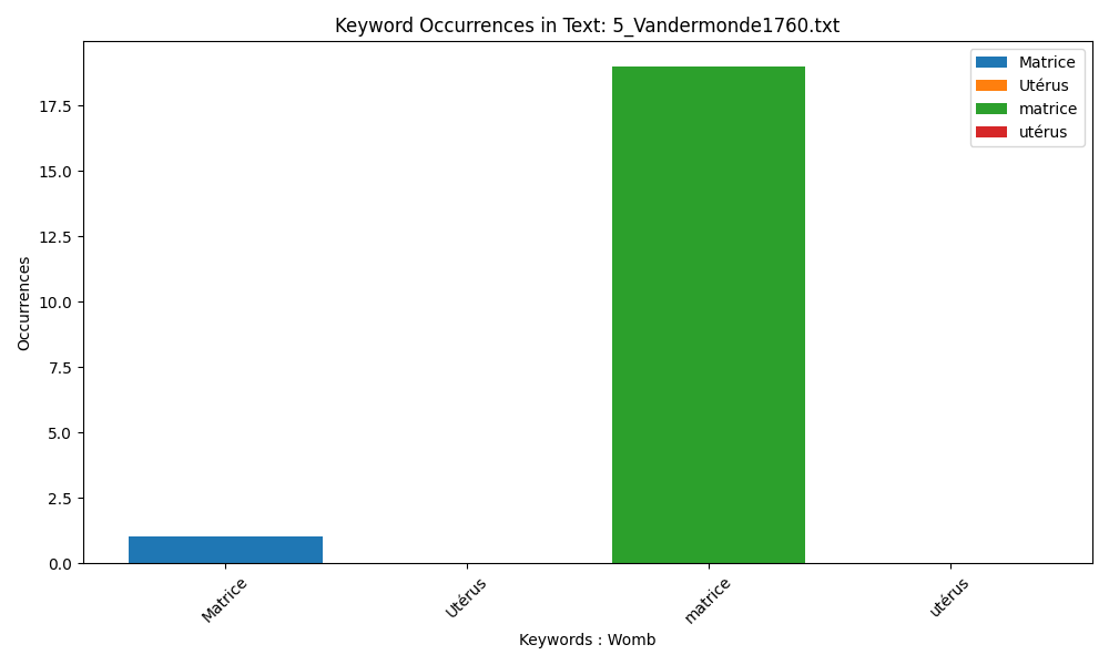
Vandermonde does in fact use ‘utérus’ but only once, writing about “les ligaments ronds de l’utérus” (1760, p. 173) under the dictionary entry for ‘Descente’.

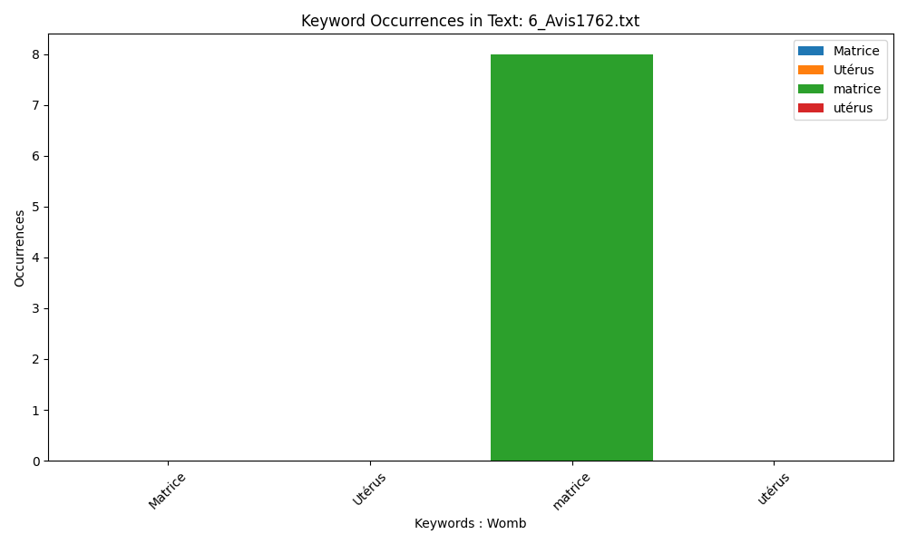
Tissot uses only ‘matrice’.

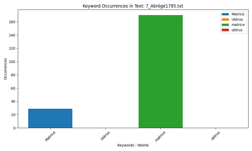
Both uppercase and lowercase are used by du Coudray.

Caveats

There are limitations to this method. The primary sources are of varying length, so the barcharts are not directly comparable in terms of trying to identify which text uses the word the most. Pages numbers could be used to standardise this information, but we worked with text files which did not maintain the page number aspect.

These .txt files are also of varying quality, depending on their original source. This means that some internal structuring issues may hinder the count, for example some words are split like th|is.

Where many sources applied differing degrees of capitalisation, we wanted to capture this. This means that this method may take in occurrences of the word where it appears at the start of a sentence; however given that they are nouns, this is somewhat unlikely.

Python

WombTerms_FR

In [2]:

import os
import glob
import matplotlib.pyplot as plt
from nltk.tokenize import word_tokenize
import nltk
nltk.download('punkt')  # Download the necessary resource for tokenization

# Step 1: Read the text files from the folder
folder_path = 'text_pythonFR'
text_files = glob.glob(os.path.join(folder_path, '*.txt'))

# List of manually selected keywords
selected_keywords = ['Matrice', 'Utérus', 'matrice', 'utérus']

# Initialize a dictionary to store keyword occurrences per text
text_keyword_occurrences = {keyword: [] for keyword in selected_keywords}

# Step 2: Tokenize the text into words and count occurrences
for file_path in text_files:
    with open(file_path, 'r', encoding='utf-8') as file:
        text = file.read()
        words = word_tokenize(text)
        
        # Count keyword occurrences in the text
        keyword_counts = {keyword: words.count(keyword) for keyword in selected_keywords}
        
        # Store keyword occurrences for the text
        for keyword in selected_keywords:
            text_keyword_occurrences[keyword].append(keyword_counts[keyword])

# Step 3: Create and save a bar chart for each individual text
output_folder = 'barcharts_FR'  # Set the path where you want to save the charts

for file_path in text_files:
    text_name = os.path.basename(file_path)
    
    plt.figure(figsize=(10, 6))
    for keyword in selected_keywords:
        plt.bar(keyword, text_keyword_occurrences[keyword][text_files.index(file_path)], label=keyword)
    
    plt.xlabel('Keywords : Womb')
    plt.ylabel('Occurrences')
    plt.title(f'Keyword Occurrences in Text: {text_name}')
    plt.legend()
    plt.xticks(rotation=45)
    plt.tight_layout()
    
    # Save the bar chart as an image
    chart_file_name = os.path.splitext(text_name)[0] + '_chart.png'
    chart_file_path = os.path.join(output_folder, chart_file_name)
    plt.savefig(chart_file_path)
    
    # Display the bar chart (optional)
    plt.show()

[nltk_data] Downloading package punkt to
[nltk_data]     C:\Users\falle\AppData\Roaming\nltk_data...
[nltk_data]   Package punkt is already up-to-date!